Projector Calibration
This tutorial describes how you can calibrate a telecentric, collimated and lens (perspective) projector.
Trace single projector pixels
Dr.TVAM has the option to trace single rays instead of doing an optimization.
The following example shows how to trace rays for a single projector pixel for each of the systems
Here we specify the different projector types: collimated, telecentric and lens.
The pixel size in object space is each 0.01mm and the resolution of the projector is 1000x1000 pixels.
The qualitative difference between the three projector types is shown in the figure below.
In the collimated case, rays are always parallel and do not diverge.
In the telecentric case, rays are parallel but do diverge with a certain angle according to the aperture radius and focus distance.
In the lens case, rays are diverging according to the aperture radius and focus distance, but they are not parallel.


Config file to trace single rays collimated (click to expand)
{
"vial": {
    "type": "cylindrical",
    "r_int": 16.363,
    "r_ext": 17.354,
    "ior": 1.00,
    "medium": {
        "ior": 1.00,
        "extinction": 0.11512925464970229,
        "albedo": 0.0
    }
},
"projector": {
    "type": "collimated",
    "n_patterns": 1,
    "resx": 1000,
    "resy": 1000,
    "pixel_size": 10e-3,
    "motion": "circular",
    "distance": 50
},
"sensor": {
    "type": "dda",
    "scalex": 10,
    "scaley": 10,
    "scalez": 10,
    "film": {
        "type": "vfilm",
        "resx": 256,
        "resy": 256,
        "resz": 1
    }
},
"target": {
    "filename": "cylinder.ply",
    "size": 1000
},
"psf_analysis": [
    {
        "x": 500,
        "y": 500,
        "index_pattern": 0,
        "intensity": 1000
    },
    {
        "x": 400,
        "y": 500,
        "index_pattern": 0,
        "intensity": 1000
    },
    {
        "x": 300,
        "y": 500,
        "index_pattern": 0,
        "intensity": 1000
    },
    {
        "x": 200,
        "y": 500,
        "index_pattern": 0,
        "intensity": 1000
    },
    {
        "x": 100,
        "y": 500,
        "index_pattern": 0,
        "intensity": 1000
    },
    {
        "x": 0,
        "y": 500,
        "index_pattern": 0,
        "intensity": 1000
    },
    {
        "x": 600,
        "y": 500,
        "index_pattern": 0,
        "intensity": 1000
    },
    {
        "x": 700,
        "y": 500,
        "index_pattern": 0,
        "intensity": 1000
    },
    {
        "x": 800,
        "y": 500,
        "index_pattern": 0,
        "intensity": 1000
    },
    {
        "x":900,
        "y": 500,
        "index_pattern": 0,
        "intensity": 1000
    }
],
"spp_ref": 8000
}
Config file to trace single rays telecentric (click to expand)
{
 "vial": {
     "type": "cylindrical",
     "r_int": 16.363,
     "r_ext": 17.354,
     "ior": 1.00,
     "medium": {
         "ior": 1.00,
         "extinction": 0.11512925464970229,
         "albedo": 0.0
     }
 },
 "projector": {
     "type": "telecentric",
     "n_patterns": 1,
     "resx": 1000,
     "resy": 1000,
     "pixel_size": 10e-3,
     "motion": "circular",
     "distance": 50,
     "focus_distance": 50,
     "aperture_radius": 2
 },
 "sensor": {
     "type": "dda",
     "scalex": 10,
     "scaley": 10,
     "scalez": 10,
     "film": {
         "type": "vfilm",
         "resx": 256,
         "resy": 256,
         "resz": 1
     }
 },
 "target": {
     "filename": "cylinder.ply",
     "size": 1000
 },
 "psf_analysis": [
     {
         "x": 500,
         "y": 500,
         "index_pattern": 0,
         "intensity": 1000
     },
     {
         "x": 400,
         "y": 500,
         "index_pattern": 0,
         "intensity": 1000
     },
     {
         "x": 300,
         "y": 500,
         "index_pattern": 0,
         "intensity": 1000
     },
     {
         "x": 200,
         "y": 500,
         "index_pattern": 0,
         "intensity": 1000
     },
     {
         "x": 100,
         "y": 500,
         "index_pattern": 0,
         "intensity": 1000
     },
     {
         "x": 0,
         "y": 500,
         "index_pattern": 0,
         "intensity": 1000
     },
     {
         "x": 600,
         "y": 500,
         "index_pattern": 0,
         "intensity": 1000
     },
     {
         "x": 700,
         "y": 500,
         "index_pattern": 0,
         "intensity": 1000
     },
     {
         "x": 800,
         "y": 500,
         "index_pattern": 0,
         "intensity": 1000
     },
     {
         "x":900,
         "y": 500,
         "index_pattern": 0,
         "intensity": 1000
     }
 ],
 "spp_ref": 8000
 }
Config file to trace single rays lens (click to expand)
{
"vial": {
    "type": "cylindrical",
    "r_int": 16.363,
    "r_ext": 17.354,
    "ior": 1.00,
    "medium": {
        "ior": 1.00,
        "extinction": 0.11512925464970229,
        "albedo": 0.0
    }
},
"projector": {
    "type": "lens",
    "n_patterns": 1,
    "resx": 1000,
    "resy": 1000,
    "pixel_size": 10e-3,
    "motion": "circular",
    "distance": 50,
    "focus_distance": 50,
    "aperture_radius": 2
},
"sensor": {
    "type": "dda",
    "scalex": 10,
    "scaley": 10,
    "scalez": 10,
    "film": {
        "type": "vfilm",
        "resx": 256,
        "resy": 256,
        "resz": 1
    }
},
"target": {
    "filename": "cylinder.ply",
    "size": 1000
},
"psf_analysis": [
    {
        "x": 500,
        "y": 500,
        "index_pattern": 0,
        "intensity": 1000
    },
    {
        "x": 400,
        "y": 500,
        "index_pattern": 0,
        "intensity": 1000
    },
    {
        "x": 300,
        "y": 500,
        "index_pattern": 0,
        "intensity": 1000
    },
    {
        "x": 200,
        "y": 500,
        "index_pattern": 0,
        "intensity": 1000
    },
    {
        "x": 100,
        "y": 500,
        "index_pattern": 0,
        "intensity": 1000
    },
    {
        "x": 0,
        "y": 500,
        "index_pattern": 0,
        "intensity": 1000
    },
    {
        "x": 600,
        "y": 500,
        "index_pattern": 0,
        "intensity": 1000
    },
    {
        "x": 700,
        "y": 500,
        "index_pattern": 0,
        "intensity": 1000
    },
    {
        "x": 800,
        "y": 500,
        "index_pattern": 0,
        "intensity": 1000
    },
    {
        "x":900,
        "y": 500,
        "index_pattern": 0,
        "intensity": 1000
    }
],
"spp_ref": 8000
}
Notable we introduce a psf_analysis section in the JSON file.
This section contains a list of rays to be traced. Each ray is defined by its x and y pixel coordinates, the index_pattern (which pattern to use), and the intensity of the ray.
If drtvam config.json is run, it will only trace the rays defined in the psf_analysis section.
The output intensity traces are written in final.exr and final.npy. The pixel size of the output is defined by the sensor,
hence the output will be 256x256 pixels in this case with a space resolution of 0.039mm
Since the refractive index of the vial is 1.0, the rays will not be refracted and will travel in a straight line, as expected in air.
The rays are attenuated by the extinction coefficient of the medium, which is set to 0.115.
The target is irrelevant for this example, but it is required to run the simulation.
We shoot a total of 8000 rays per pixel, as defined by the spp_ref parameter. It is possible to change this value to increase or decrease the number of rays per pixel. It makes the results more accurate.
Note, in an optimization, increasing the spp parameters to such high values, will result in very long optimizations.
So values around 100 (spp=100, spp_ref=100 and spp_grad=100) are more realistic and sufficient for most applications.
Calibration a real lens projector
This example shows how to calibrate a real lens projector setup.
The parameters for such a projector are resx, resy, fov, aperture_radius, focus_distance and distance.
A sketch of the parameters is given in this figure.

The challenge in the calibration is to find the parameters aperture_radis, focus_distance and distance. The fov indicates the field of view in the image plane in x direction in degrees.
This can be simply measured by a ruler.
But since the fov also depends on the distance, it is intertwisted with the other parameters. The aperture_radius is the radius of the aperture which describes how large the light cone
is going to be. Note, this is a abstract, conceptualized projector so the aperture radius is not the physical aperture of a lens, but rather a parameter that describes the light cone of the projector which also depends on your illumination source.
But focus_distance is the roughly the distance from the lens to the focal plane, which is the plane where the rays are focused.
The following config files generates the traces of singles rays through a cylindrical vial filled with a medium.
Config file lens projector (click to expand)
{
    "vial": {
        "type": "cylindrical",
        "r_int": 6.363,
        "r_ext": 7.354,
        "ior": 1.54,
        "medium": {
            "ior": 1.4847,
            "phase": {
                "type": "rayleigh"
            },
            "extinction": 0.11512925464970229,
            "albedo": 0.0
        }
    },
    "projector": {
        "type": "lens",
        "n_patterns": 1,
        "resx": 740,
        "resy": 700,
        "fov": 5.57,
        "aperture_radius": 2.1,
        "focus_distance":  152,
        "motion": "circular",
        "distance": 150
    },
    "sensor": {
        "type": "dda",
        "scalex": 18.90,
        "scaley": 18.90,
        "scalez": 18.90,
        "film": {
            "type": "vfilm",
            "resx": 1000,
            "resy": 1000,
            "resz": 1
        }
    },
    "target": {
        "filename": "cylinder.ply",
        "size": 1000
    },
    "psf_analysis": [
        {
            "x": 370,
            "y": 350,
            "index_pattern": 0,
            "intensity": 1
        },
        {
            "x": 270,
            "y": 350,
            "index_pattern": 0,
            "intensity": 1
        },
        {
            "x": 170,
            "y": 350,
            "index_pattern": 0,
            "intensity": 1
        },
        {
            "x": 470,
            "y": 350,
            "index_pattern": 0,
            "intensity": 1
        },
        {
            "x": 570,
            "y": 350,
            "index_pattern": 0,
            "intensity": 1
        },
        {
            "x": 670,
            "y": 350,
            "index_pattern": 0,
            "intensity": 1
        },
        {
            "x": 70,
            "y": 350,
            "index_pattern": 0,
            "intensity": 1
        }

    ],
    "spp_ref": 8000
}
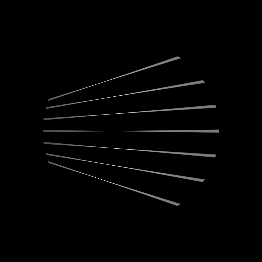
Running drtvam this_config.json will generate the traces of the rays through the vial. The output in final.exr should look like this:
In experiment we capture similar traces through a glass vial filled with a medium. To make the trace visible we use fluorescent dye in the medium. It is important to determine the pixel size of the experimental camera in the focal plane (your imaging system might be not telecentric). Further, the projected pixels in the real setup should hit the vial as close as possible to the vertical end of the vial. Otherwise there is geometric distortion in the image because of the refractive index mismatch between the medium and the air. We then overlay the experimental image with the simulated traces to find the best fit of the simulated traces to the experimental image. The strategy is to rotate and move (do not scale) the setup image over the simulated traces until the best fit is found. Then we save the experimental image as new picture. With the following Python script we can overlay the experimental image with the simulated traces.
Helper script to overlay experimental image with simulated traces (click to expand)
import matplotlib.pyplot as plt
import numpy as np
import imageio

# last dimension is singleton and has no meaning
img = np.load('final.npy')[:, :, :, 0]

img_from_top = np.sum(img, axis=0)

# here we should load our reference images from the real setups
# load setup.bmp
img_from_top_setup = imageio.imread('setup.bmp')


# plot the images and also make another row with overlay images
# top with setup each. Overlay in matplotlib with alpha and colors
plt.figure(figsize=(10, 5))
plt.subplot(1, 3, 1)
plt.imshow(img_from_top)
plt.title('Image from Top')
plt.subplot(1, 3, 2)
plt.imshow(img_from_top_setup, alpha=0.5, cmap='gray')
plt.title('Image from Setup')

# overlay
plt.subplot(1, 3, 3)
plt.imshow(img_from_top_setup, cmap='gray')
plt.imshow(img_from_top, alpha=0.5, cmap='jet')
plt.title('Overlay Image')

plt.tight_layout()
plt.show()
With the following helper script, we can overlay the experimental image with the simulated traces. By running drtvam and adapting the parameters, we can find the best fit of the simulated traces to the experimental image.
The resulting image is shown in the figure below.
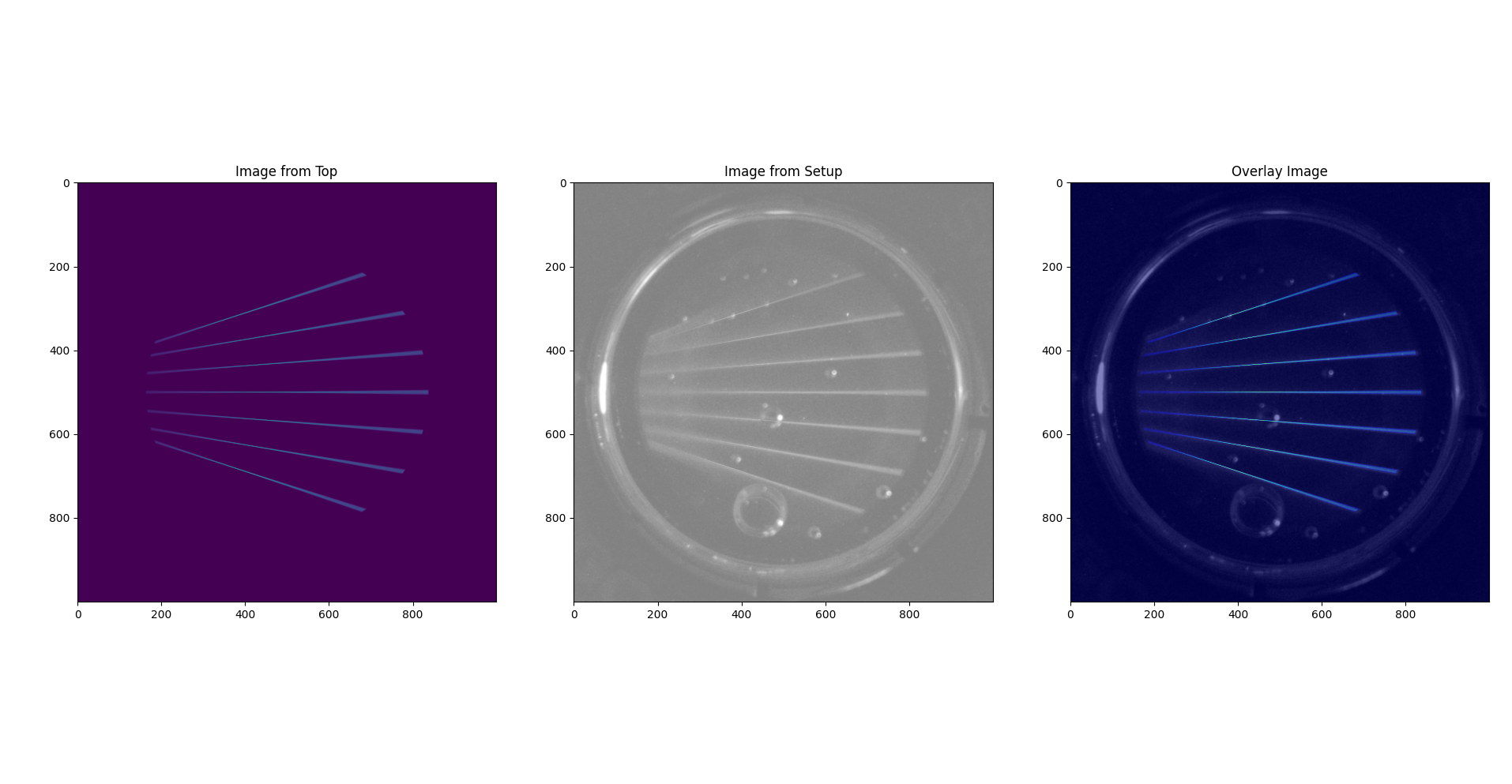
By tweaking the parameters in the config file and running drtvam config_psf.json; python overlay.py we can find the best fit of the simulated traces to the experimental image in a couple of iterations.
Calibration of a collimated projector
The calibration of a collimated projector is trivial as the only required property is the pixel_size of the projector in image plane.
This can be easily measured with a detector or ruler.
Calibration of a telecentric projector
The calibration of a telecentric projector is more work than the collimated projector, but less than the lens projector.
Additionally to the pixel_size, the distance, aperture_radius and focus_distance are required. These can be easily inferred from
an experimental capture image from top (or bottom) through a vial filled with a medium.